Headphones Test Bench 2.2 archived this test and retired the waterfall plot visualization from our testing suite. Please see the changelog for more information.
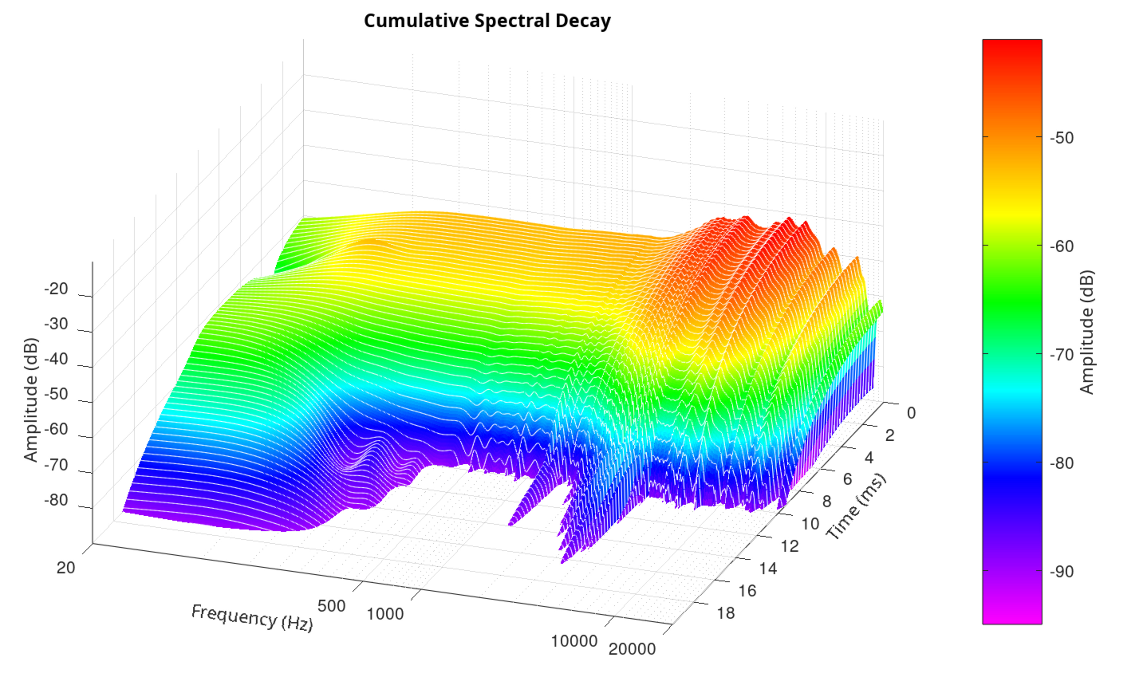
Cumulative Spectral Decay (CSD) plots are a well-established way to evaluate how acoustic transducers handle resonances and decay. They look impressive and promise insight into "ringing" and system behavior, but they can also be misleading if not interpreted carefully.
Thanks to requests from readers like you, in our headphones 2.0 test bench, we've published over 40 CSD plots and conducted extensive internal testing. Through this process, we've identified significant variability in the results, much of which has little to do with the headphones themselves. To make this issue concrete, this article will use the Sennheiser HD 800 S as a case study to explore the reliability and limitations of CSD analysis in the context of headphones.
While CSD is a powerful tool in loudspeaker testing, where reflections and decay times correspond to real acoustic distances, its meaning in headphone analysis is far less grounded. In the tightly coupled acoustic space between a headphone driver and the ear, there are no significant reflections or reverberation. In this context, "decay" is shaped less by physical behavior and more by analysis settings. What looks like a lingering resonance might, in fact, be a windowing artifact.
To illustrate this, below are four CSD plots of the same HD 800 S impulse response, processed with different windowing settings:
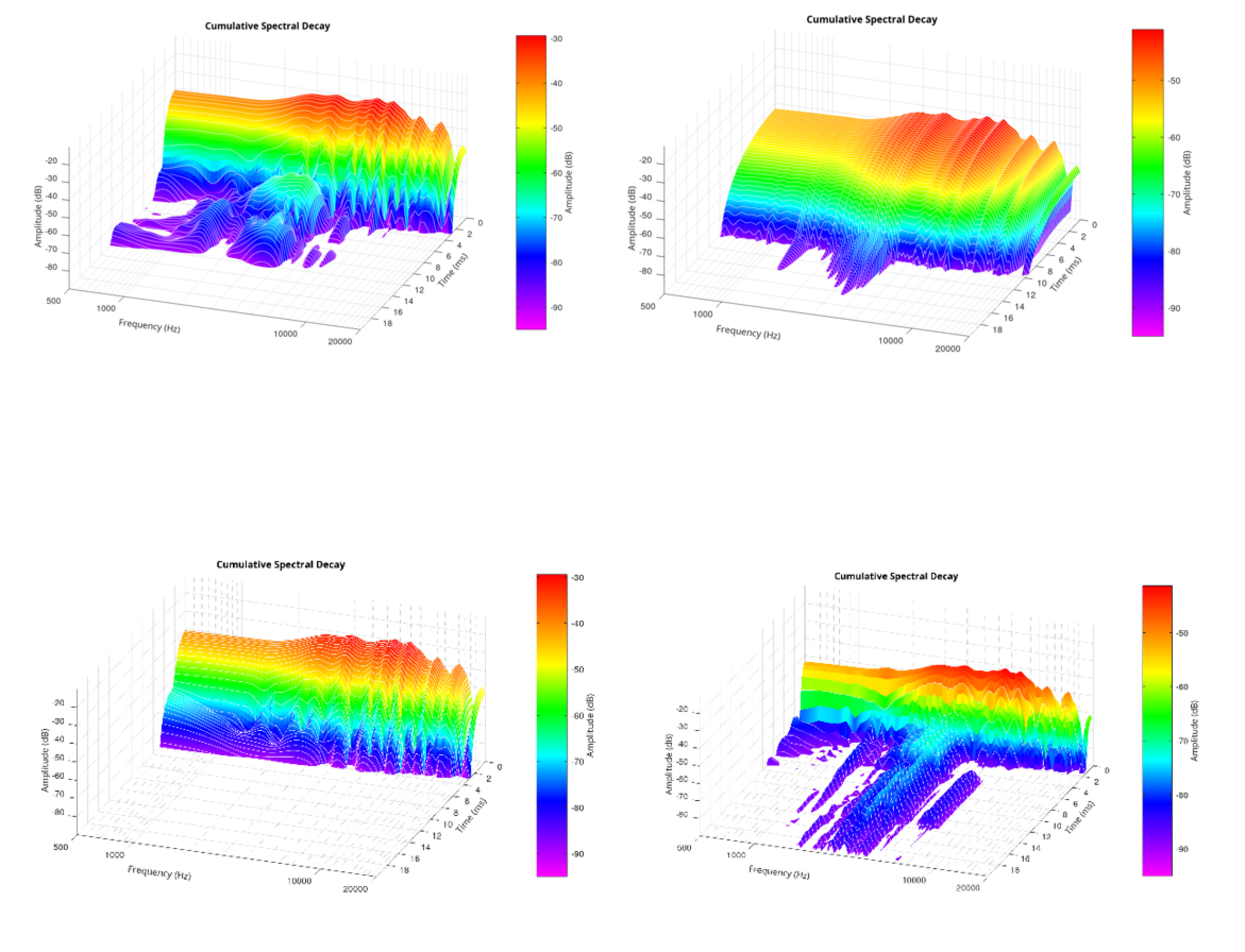
Each graph tells a different story—yet the transducer hasn't changed. Whether it's a shift in window type, length, or slice count, the outcome shifts dramatically. This striking variability reveals a central truth: CSD plots often reflect the measurement method more than the device under test.
How CSDs Are Made
Let's walk through the basic process of creating a CSD graph.
Like with frequency response measurements, all the necessary data is embedded in the system's impulse response, which is extracted from a logarithmic frequency sweep. This sweep ramps from low to high frequencies and is played back through the headphones. Once the analyzer records the system's output, a deconvolution is applied, which time-reverses and amplitude-compensates the sweep, effectively "undoing" it and isolating the system's impulse response. In frequency terms, it's just output divided by input.
From there comes the Short-Time Fourier Transform (STFT). This technique slices the impulse response into small, overlapping time segments and runs a Fast Fourier Transform (FFT) on each one. This allows the visualization of how frequency content changes over time.
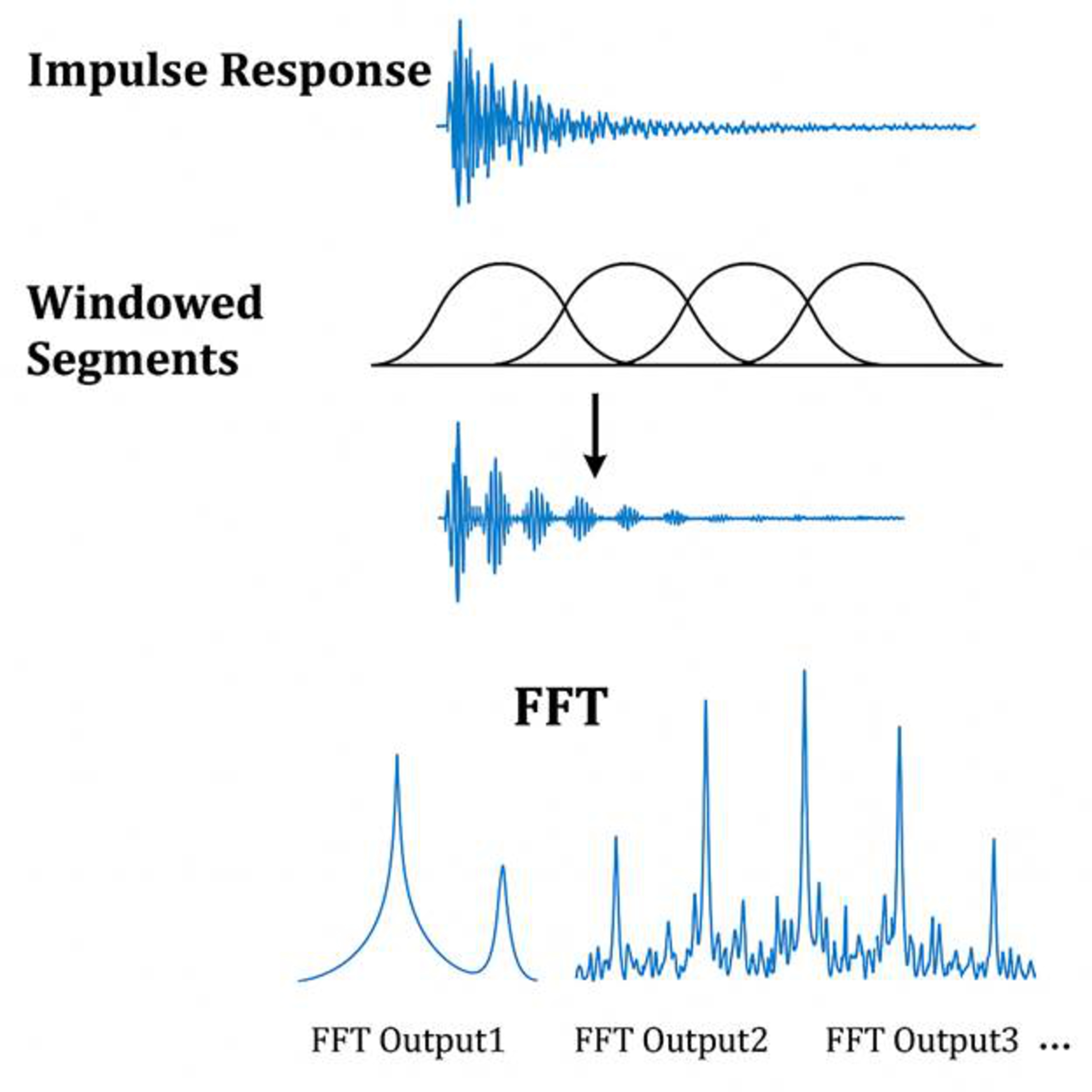
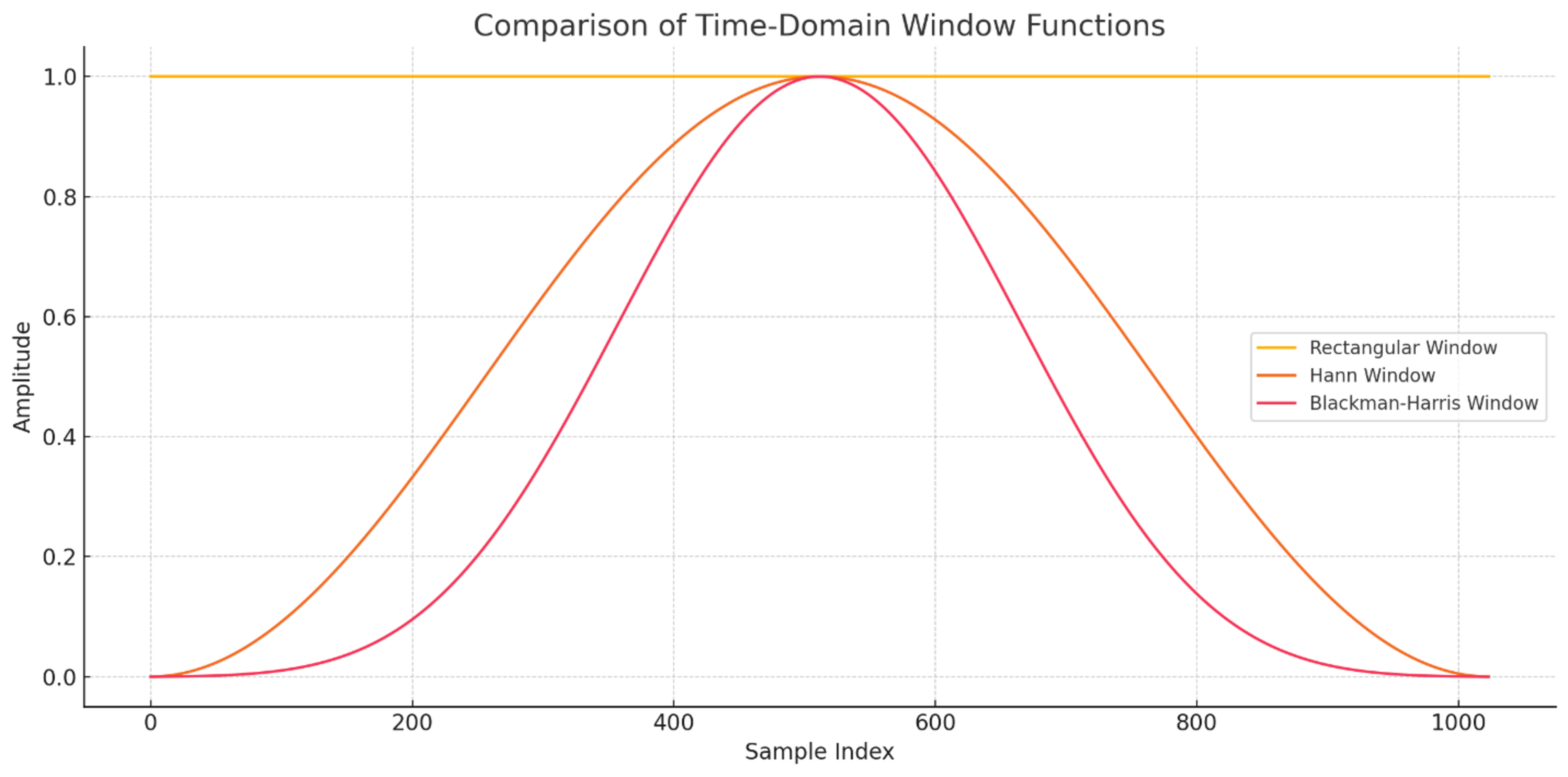
To reduce artifacts, each segment is shaped with a window function—a taper that softens the start and end of the segment to minimize sharp transitions. Tapered windows like Hann, Hamming, and Blackman-Harris reduce spectral leakage (energy spilling into neighboring frequencies), but they also reduce the apparent amplitude and blur short-lived events. A rectangular window applies no tapering, giving better time resolution but at the cost of high leakage.
Here's how they look:
The final CSD is built by stacking the spectral snapshots over time: frequency on the X-axis, time on the Y-axis, and amplitude (in dB) as a color gradient or Z-axis. The result is a waterfall plot that reveals how energy decays at each frequency.
FFT Length, Frequency Bins, Time Windows, and Slicing
Each CSD plot is shaped by four key parameters that define how the STFT is computed:
- FFT Length (NFFT): This defines the number of points used in the FFT. A larger FFT increases frequency resolution, meaning narrower frequency bins and better visibility of fine spectral details. However, it also smooths over time, blurring fast transients. On the flip side, a shorter FFT gives you sharper time resolution. You can pinpoint when energy appears or disappears more precisely. However, with fewer samples, the frequency bins widen, and narrow spectral features get lost.
- Frequency Bins: The FFT outputs these bins, each one representing a frequency range.
Frequency Bin Spacing (Δf):
Δf = Fs / FFT Length
Where:
- Δf is the frequency resolution (spacing between FFT bins)
- Fs is the sampling rate in Hz
- FFT Length is the number of points used in the FFT
Example:
For Fs = 192,000Hz and FFT Length = 1024:
Δf = 192,000 / 1024 = 187.5Hz
- Window Duration (Time Window Length): This is how long each time segment is. Longer windows improve frequency resolution but smear timing. Shorter windows improve temporal accuracy but reduce spectral detail. For example, at 192kHz, a 1024-sample window spans ~5.33 ms.
- Hop Size (Samples per Shift): This is how far the window slides forward between FFTs. Smaller hop sizes mean more overlapping segments, more time slices, and smoother decay tracking. In Audio Precision's CSD utility, Samples/Shift directly sets the number of time slices, independent of FFT length. For instance, 30 samples/shift might yield 86 slices, and 31 might yield 91, regardless of whether the FFT size is 512 or 1024.
Together, these parameters determine the resolution tradeoff in your CSD: whether you see a precise breakdown of frequencies, a clear sense of timing, or a compromise between both. That's at least the theory, but we'll see later that it's not the end of it.
How we do it
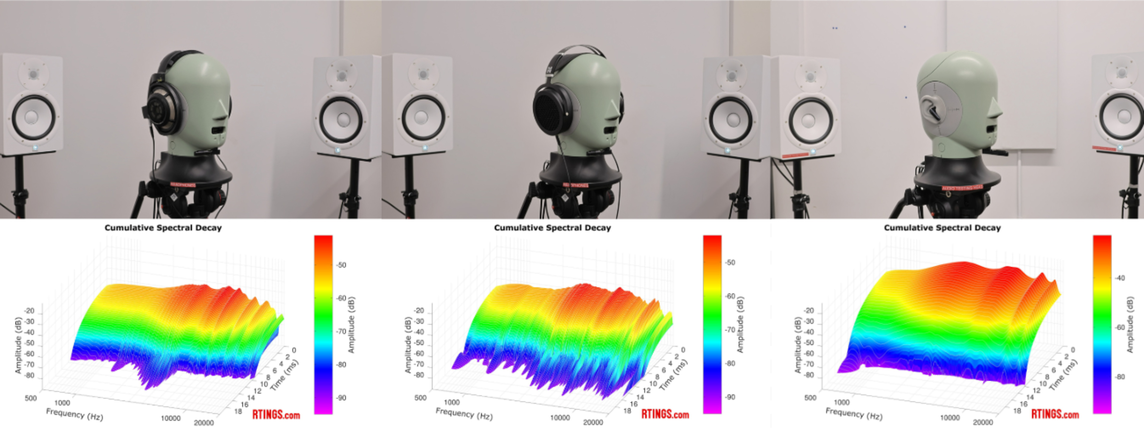
At RTINGS.com, we generate CSD plots using the Audio Precision platform, which gives us practical control over how the impulse response is segmented and analyzed, based on the principles covered earlier, but with implementation-specific tools.
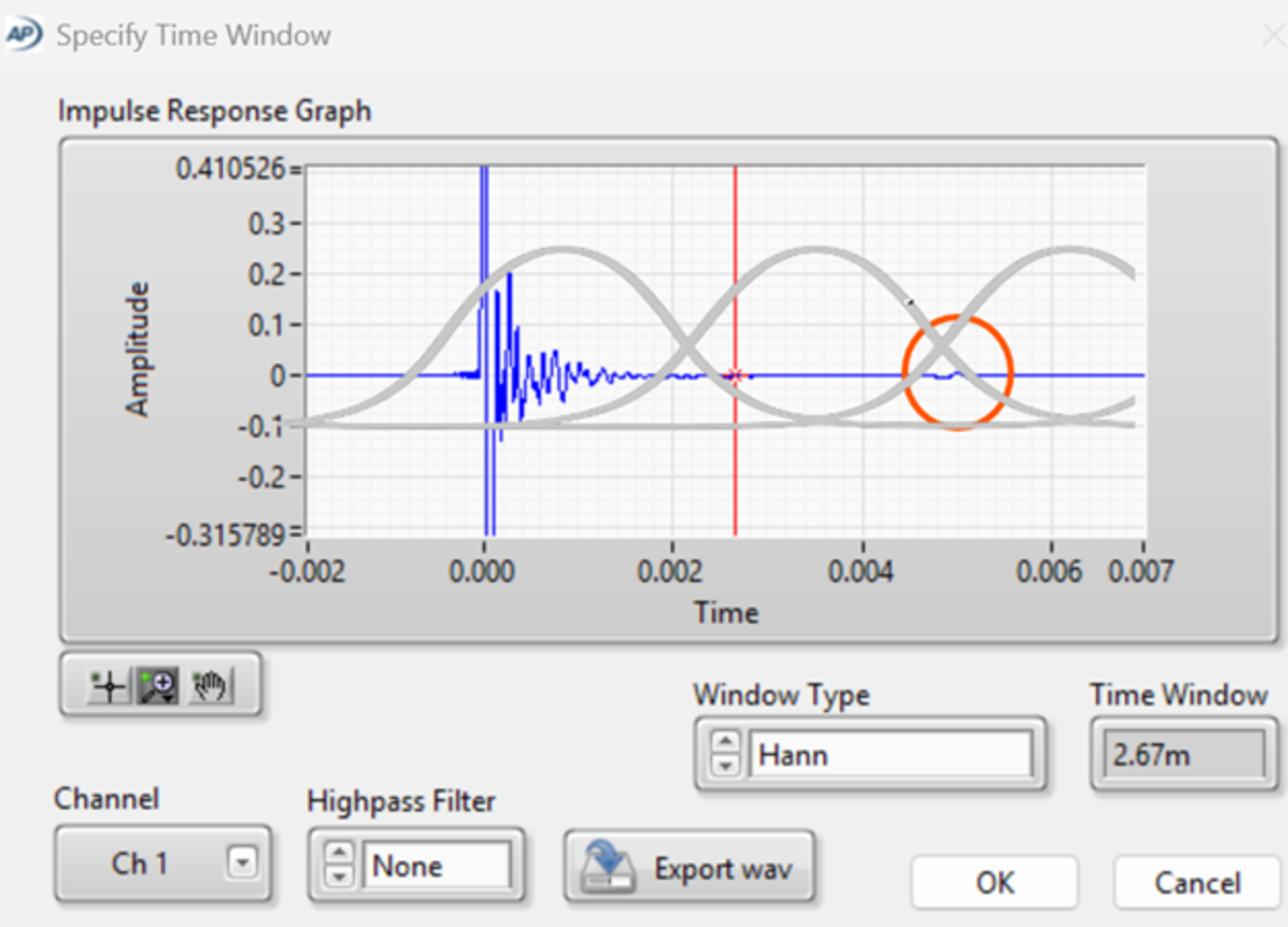
There are two main windowing modes available:
- Hann Window uses a fixed taper shape with parameters like window length, FFT size, and samples per shift. This last one directly controls how many slices are produced by defining how much the window moves per step.
- Rectangular + Tapers allow explicit control over window duration, rise time (i.e., tapering at the edges), and number of slices. These parameters affect both frequency and time resolution and influence the visibility of resonances.
Here's a look at the interface:
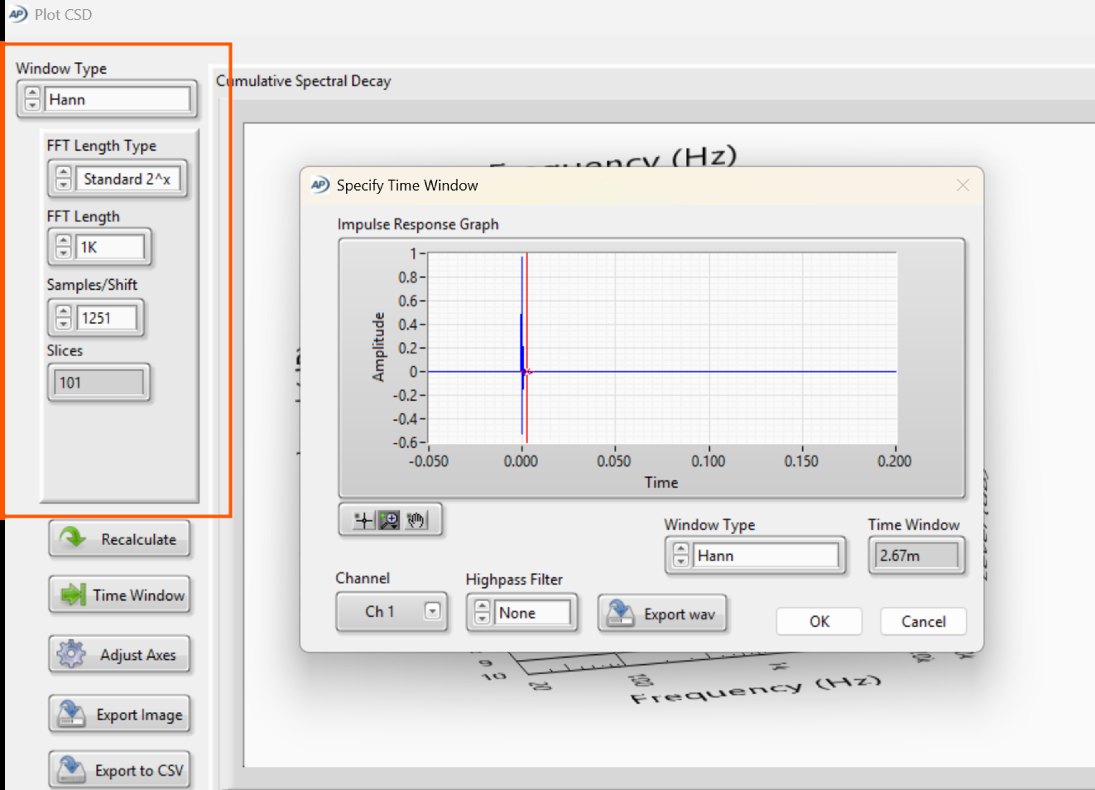
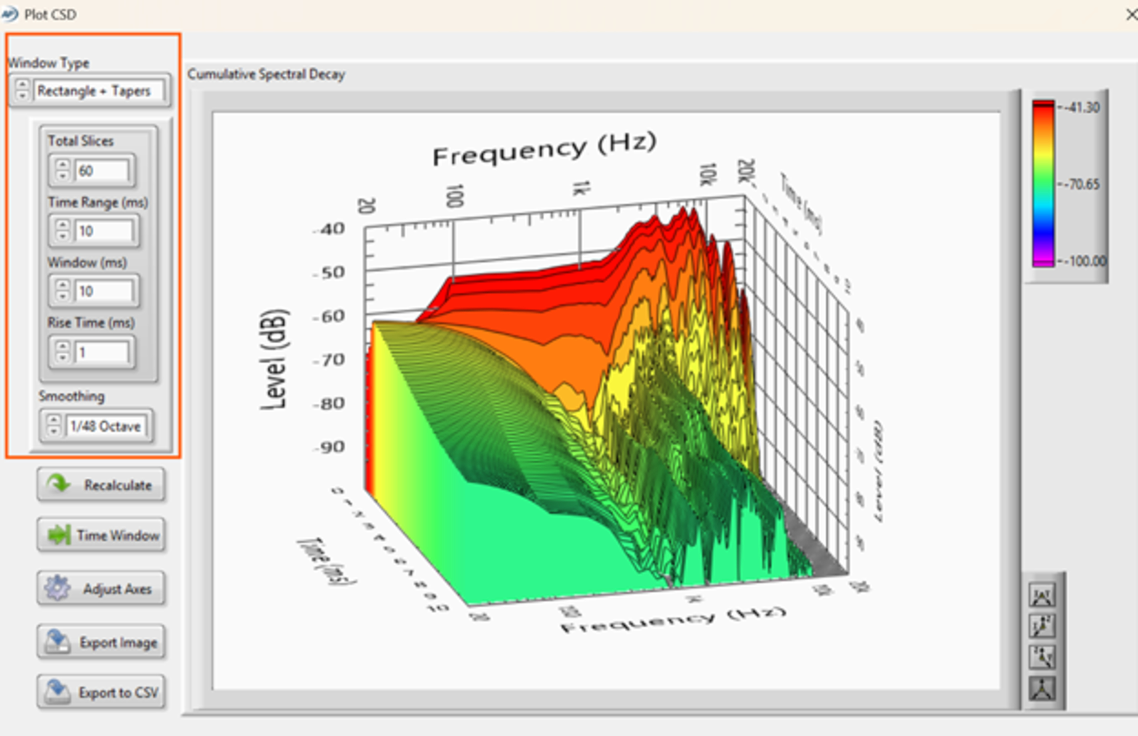
Unlike general STFT workflows, Audio Precision decouples certain parameters, like allowing high slice counts regardless of FFT size, or shaping time windows independently of the FFT. This flexibility is powerful, but it also means results can vary significantly depending on user input.
Case Study: The Sennheiser HD 800 S
To illustrate just how much these settings influence the outcome, we've included four example CSD plots using different combinations of window types, durations, and slice counts.
Hann Window – 10.61 ms, FFT size 1024, 60 slices: Moderate resolution and decay smoothness.
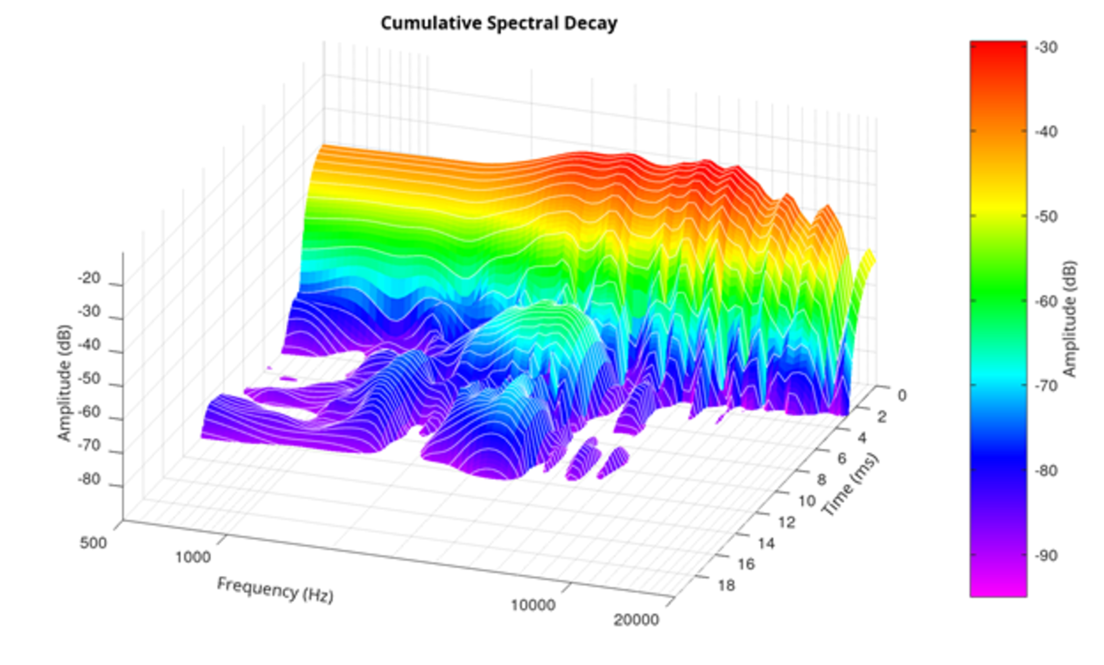
This plot uses a moderate slice count with a relatively long analysis window. While the 10.61 ms Hann window is sufficient to capture longer decays, the lower number of slices results in larger time steps between each FFT, about 0.29 ms per slice. This coarse time resolution creates blocky decay steps and makes the midrange resonances appear fluctuating or unstable.
Despite having the same FFT size and window duration as the next configuration, the difference in overlap (fewer time slices) causes more abrupt transitions between time steps, leading to a rougher and slightly noisier plot.
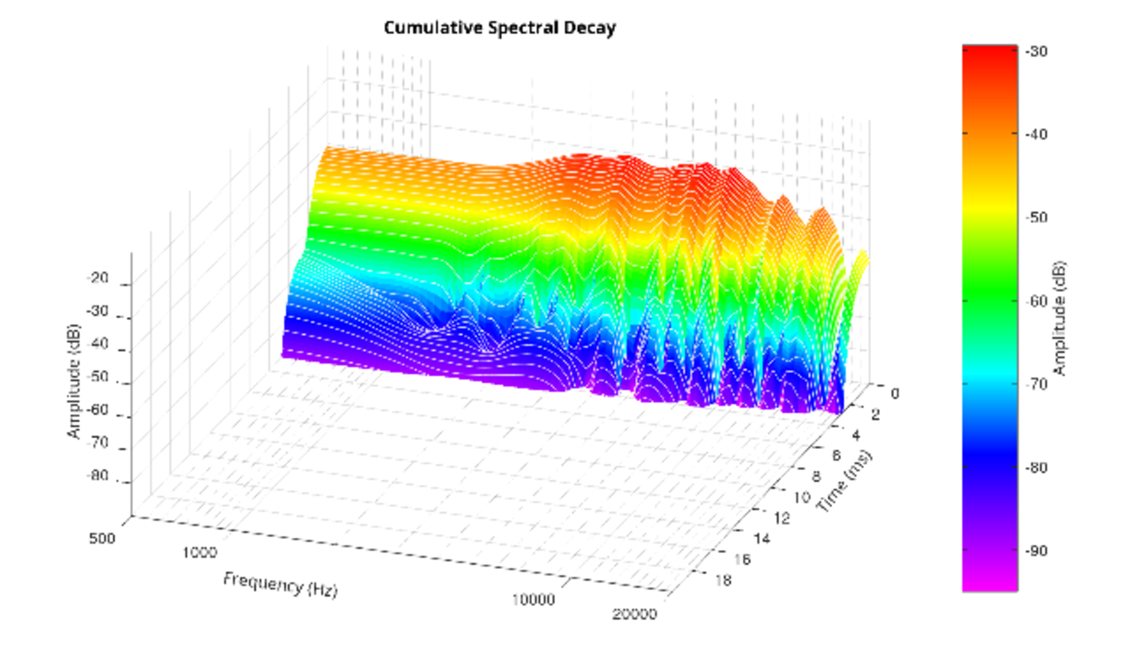
Hann Window – 10.7 ms, FFT size 1024, 158 slices
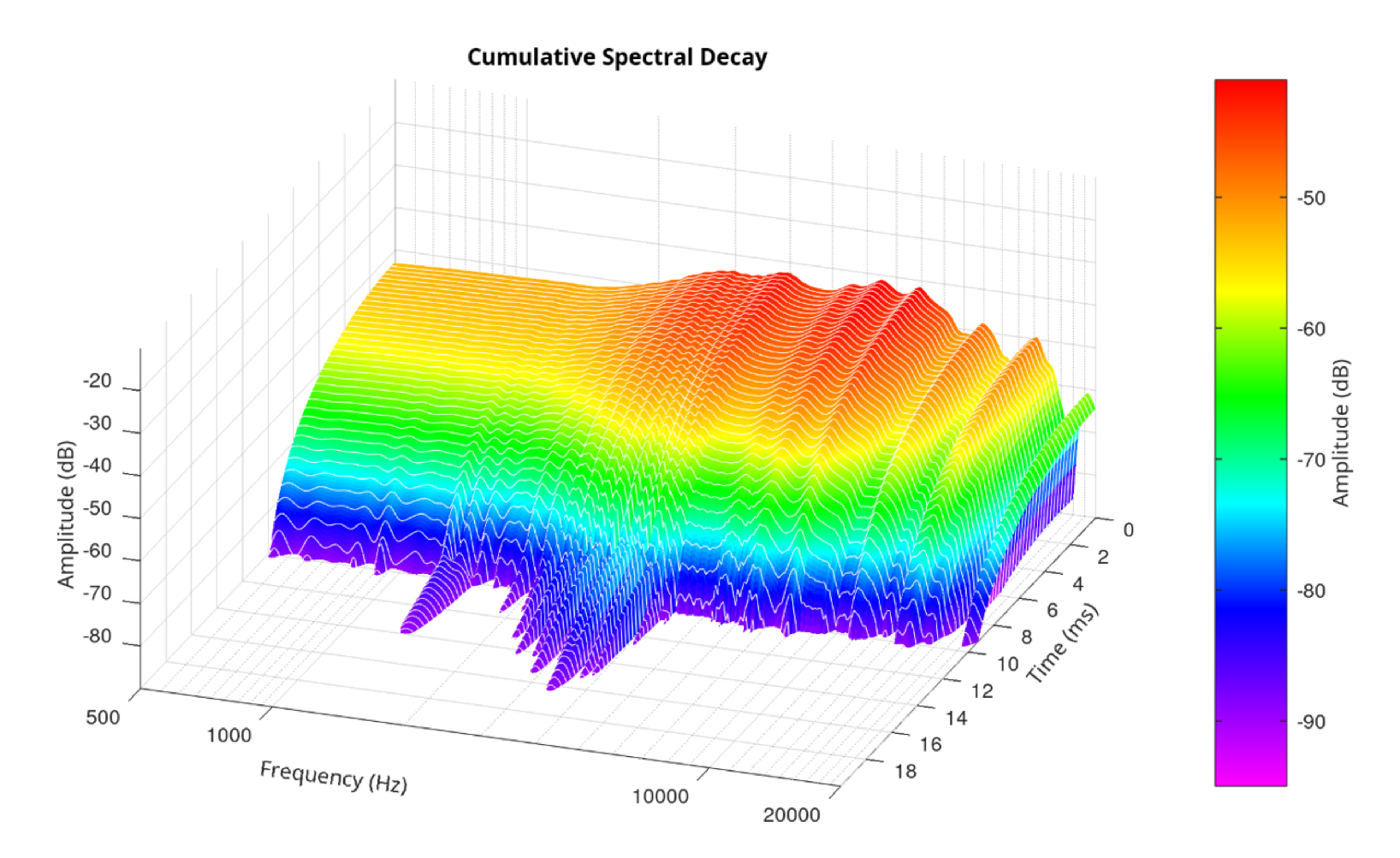
This configuration uses maximum time resolution—158 slices, the most Audio Precision allows. The analysis window length (10.7 ms) is functionally identical to the first case, but the much smaller hop size (more overlap) yields a smoother plot with clear, continuous resonances.
Midrange resonances (1.3kHz, 2–4kHz) are clearly visible and decay uniformly across time. The smoother rendering and better decay tracking are direct results of increased overlap between Hann windows. Importantly, this is also the configuration we use in our published headphone CSDs.
Why 10.7 ms? Because it corresponds to 512 samples at 44.1kHz, which is the lowest sample rate we support—critical when testing Bluetooth headphones. Even when measuring at higher rates like 96 or 192kHz, we keep this duration fixed for consistency. That way, all headphones—regardless of sample rate—are analyzed using the same observation window, ensuring comparability across models.
Hann Window – 2.67 ms, FFT size 1024, 60 slices: All visible ringing vanished.
Why Some Resonances Vanish In Shorter Windows
One of the more puzzling outcomes in CSD analysis is that, using the same impulse response and FFT size, certain resonances—especially in the midrange—can completely disappear when the window duration is shortened. So, what's happening?
To understand this, we need to clarify a few things about how CSD is computed.
In our setup, the FFT size is fixed at 1024 samples, and the sample rate is 192kHz, meaning the frequency resolution stays constant:
Δf = Fs / NFFT = 192,000 / 1024 ≈ 187.5Hz
This means each CSD slice retains the same spectral granularity whether the window is long or short.
However, what changes is the amount of temporal energy captured per slice. A Hann window of 10.7 ms (2048 samples) integrates a broader section of the impulse response, giving the FFT access to energy from longer-lasting resonances. In contrast, a shorter window—like 2.67 ms (512 samples)—ends before those decays play out fully.
You might ask: "Doesn't overlap fix that?" After all, Hann windows typically overlap significantly (often 75% or more), and our example uses 60 slices, so the time axis is densely sampled.
Yes, overlapping windows do allow the CSD to sample the impulse response more finely over time—but here's the key point:
Each individual FFT still only "sees" the energy within its own time window.
Even if a resonance decays over, say, 6–8 ms, and multiple windows overlap it, none of the windows are long enough on their own to accumulate enough energy from that decay for the resonance to stand out in the FFT. Overlap improves time tracking, not decay integration. So the energy may be "present" in the overall CSD, but never strong enough in any single slice to emerge clearly as a resonance.
On top of that, shorter windows introduce broader spectral smearing. Mathematically, windowing a signal is equivalent to convolving its spectrum with the spectrum of the window. A short Hann window produces a wide convolution kernel, which blurs narrow spectral features, like the sharp ridges caused by ringing. The resonance is not only truncated in time but smeared in frequency, further masking it from view.
In short:
- The resonance didn't vanish—it was filtered out by the analysis.
- The FFT "missed" it, not because of its size, but because the energy wasn't sustained long enough within each short segment to be measurable.
- Overlap doesn't extend the window—it just adds more snapshots with the same limits.
Here, you can see visually the effect of windowing. The resonances in the mids are a very low-level partial reflection present in the impulse. It can certainly be argued that these aren't an intrinsic part of the headphone's acoustic properties.
Rectangular + Taper – 10 ms window, 1 ms rise time, 60 slices
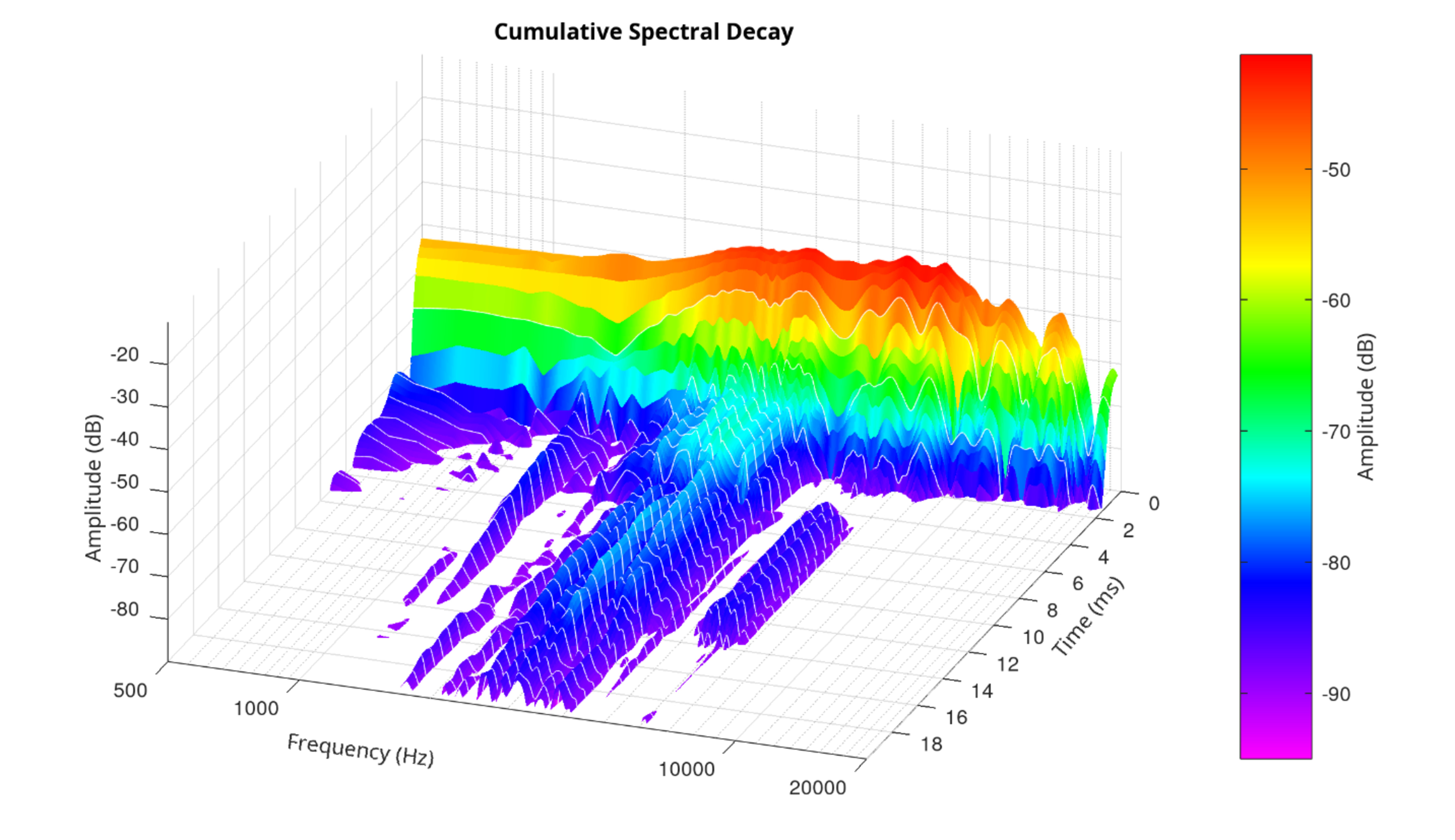
This version uses a rectangular window with a 1 ms fade-in, kind of like adding a gentle ramp at the start of the analysis slice. While rectangular windows usually preserve the full energy of a signal, the added taper in this case reduces the impact of the strongest part of the impulse.
Why? Because the fade-in begins before the impulse actually peaks. So instead of catching that initial energy head-on, it softens the front edge, effectively turning down the volume on the part that matters most. That's why this plot starts off with a noticeably lower amplitude, even though the window is technically longer than the 2.67 ms Hann.
And because the window still spans 10 ms, it collects more of the signal's tail, letting midrange resonances stretch out longer. But there's a tradeoff. Rectangular windows don't taper much in the middle, which leads to higher spectral leakage. That's why resonances in this plot look thicker and less sharply defined—they're bleeding into neighboring frequencies.
So what do we see?
- The lower starting amplitude comes from fading in too early.
- The longer decay comes from a wider time window that catches more of the tail.
- The blurry resonance bands? That's leakage from the rectangular shape doing its thing.
It's a great example of how CSDs don't just show us what the headphones are doing—they also reflect how we choose to look at it.
High Pass Filtering
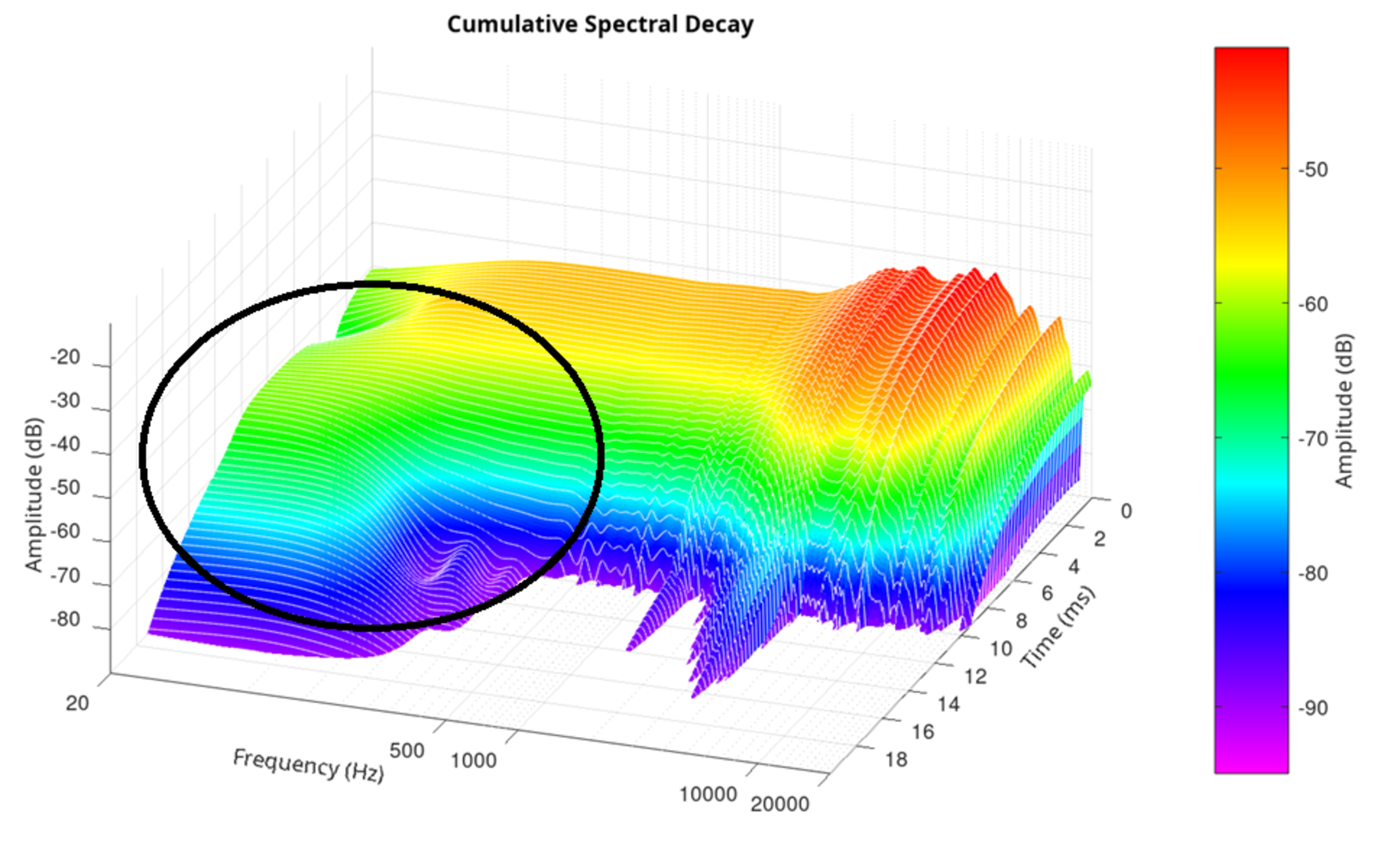
If you've looked closely at our CSD plots, you might notice something missing: the bass. We consistently filter out everything below 500Hz, and that's not a mistake—it's intentional.
Why? Because below 500Hz, all headphones start to look the same.
The decay in this range is typically broad, high in amplitude, and stretches across the entire time axis, often remaining visible past 20 milliseconds. It doesn't show distinct resonances or meaningful differences between models; it just sits there like a low-frequency fog.
This isn't necessarily a flaw in the headphones. It's a physical consequence of how bass behaves in small acoustic spaces.
At 100Hz, for example, the wavelength is over 3.4 meters, while the entire headphone cavity—driver to eardrum—is just a few centimeters. In this situation, the transducer isn't radiating into an open field or room; it's effectively pushing against a spring. That reactive load makes energy harder to dissipate quickly, and you get these long, indistinct low-frequency decays in the CSD.
Combine that with the fact that damping materials and driver design have limited effectiveness in this frequency range, and the result is a nearly universal decay smear below 500Hz.
So instead of showing a big, dark blur that tells you very little, we choose to focus our CSD plots on the 500Hz to 20kHz range, where real differences appear, resonances stand out, and windowing decisions matter.
Why CSD Plots Matter More in Loudspeaker Testing Than in Headphones
In loudspeaker measurements, CSD plots help isolate how a transducer behaves before room reflections muddy the picture. Early decay tails, windowed within a few milliseconds, correspond to real-world distances—walls, ceilings, and floor bounces. A 5 ms window might literally reflect the time before a sidewall echo hits the mic. The decay is physically grounded.
Headphones operate under very different conditions. The "room" is now just a few cubic centimeters between the driver and the ear canal. There are no distant surfaces, no late reflections—only immediate pressure variations. Nearly all of the impulse energy arrives in the first moment, leaving little room for traditional decay patterns to play out.
The effect is even more exaggerated at low frequencies, where wavelengths far exceed the dimensions of the ear cavity. At 100Hz, the wavelength is over 3.4 meters—physically too large to exhibit standing waves or reverberant decay in such a small volume.
So, what does "decay" actually represent in a headphone CSD? Likely not the acoustic environment, but rather how the measurement is windowed, tapered, and processed.
This doesn't mean headphone CSDs have no value. They can still show model-to-model differences, especially in the high end, where resonances are more localized and wavelengths are shorter. However, the visual shape of the decay is more reflective of the analysis process than the physical system.
For speakers, CSD describes an acoustic reality. For headphones, it might describe a computational one.
Are Headphones Too Predictable for CSD to Matter? The Minimum-Phase Debate
Headphones mostly behave as minimum-phase systems, meaning their phase response is in great part mathematically linked to their amplitude response. If you know the magnitude (i.e., frequency response), you can derive the phase and from there, reconstruct the time-domain decay behavior.
This raises a natural question: if decay is already encoded in the frequency response, is the CSD plot showing anything new? Or is it just a re-visualization of what we already know?
You can see again with our HD 800 S example how phase errors are also shown in the Magnitude response graph.
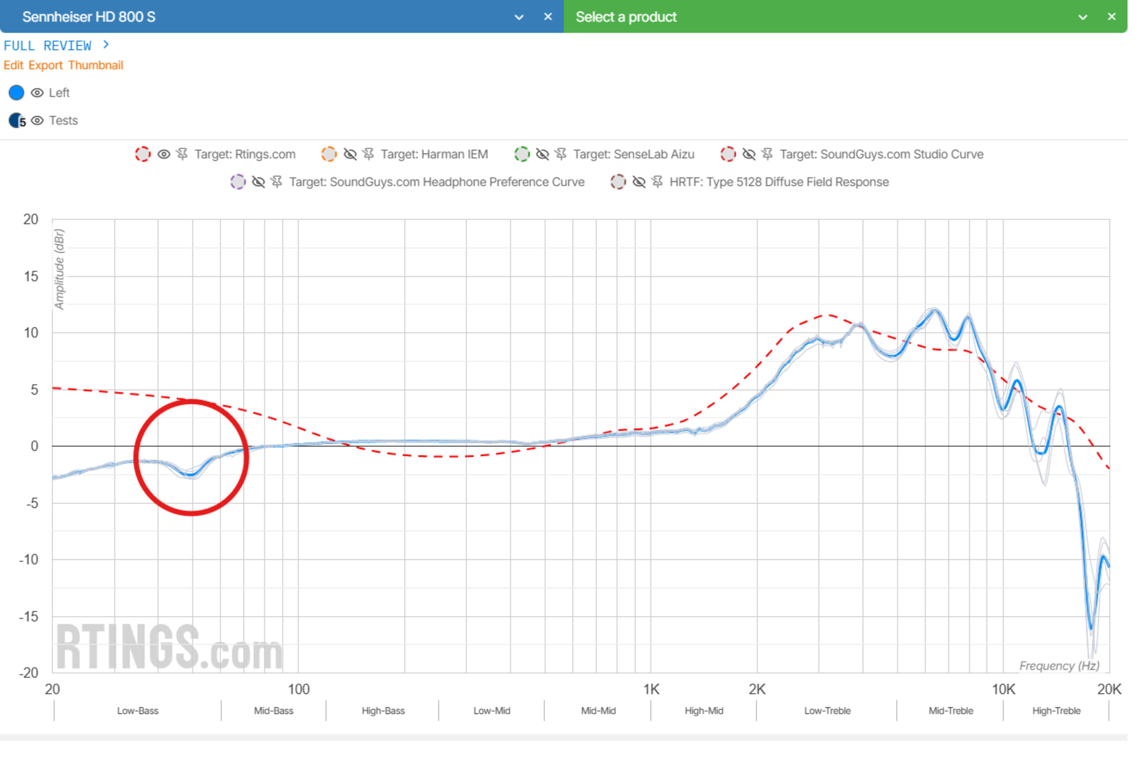
But the real issue isn't redundancy—it's variability. Because CSD relies on short-time Fourier analysis, its shape depends heavily on window length, tapering, FFT size, and slicing strategy. A different set of parameters, even from the same impulse response, can completely alter the plot. In a minimum-phase system, this means we're not necessarily visualizing a physical decay—we may be shaping a mathematical artifact.
CSDs should not be mistaken for a direct representation of a headphone's transient behavior. It's a byproduct of how the data is analyzed, not necessarily how the system sounds or performs.
This is why we believe CSD for headphones should be viewed critically and in context. While it may help illustrate how a system retains or releases energy over time, it's not a reliable standalone performance metric, especially when the underlying system is already mathematically predictable.
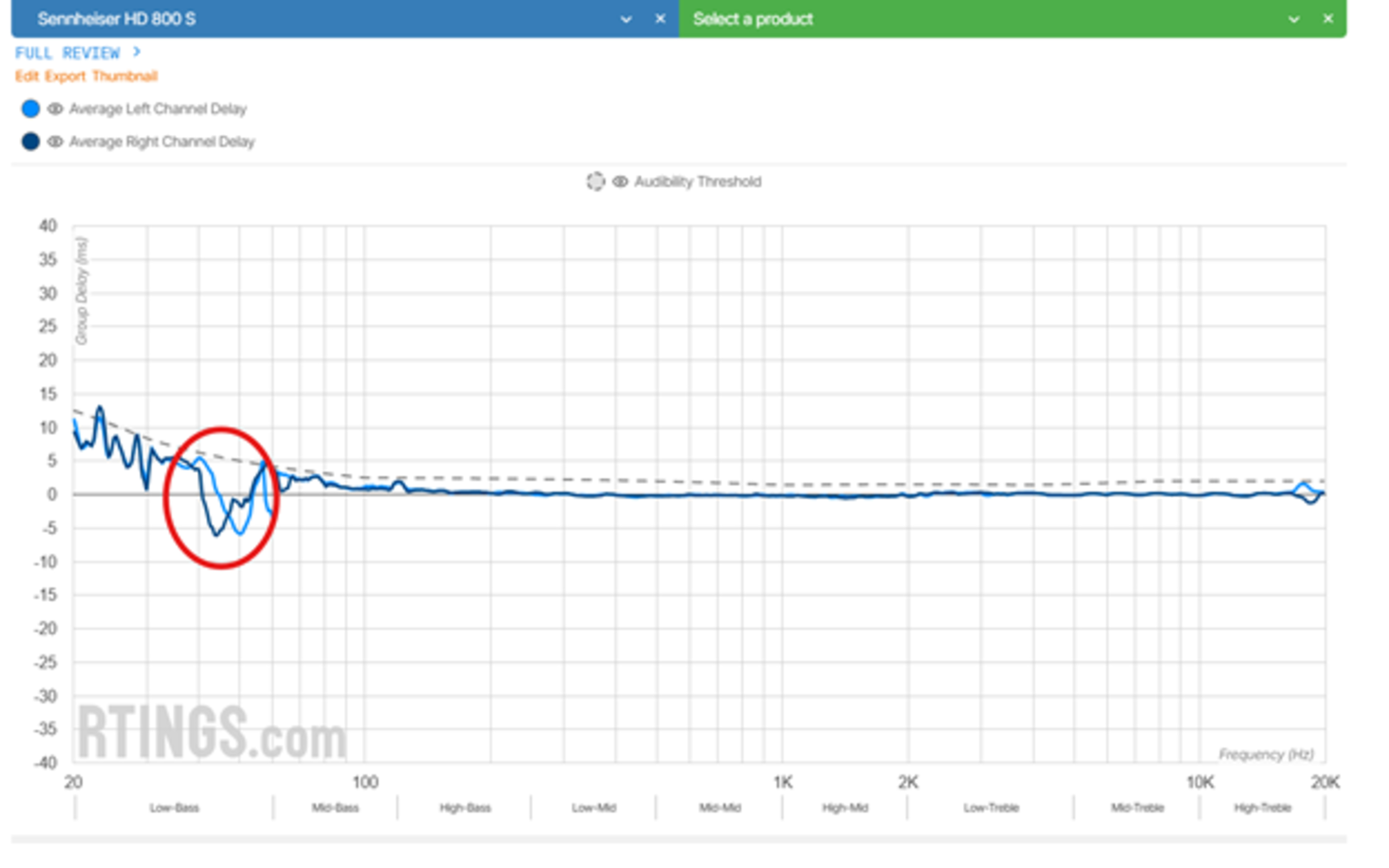
Group Delay and CSD: Shouldn't They Align?
So, going back to the minimum phase behavior of headphone transducers. In theory, this makes group delay and CSD two different ways of viewing the same time-domain behavior, so shouldn't they agree?
In practice, they don't.
In our tests, we found little to no correlation between group delay peaks and visible decay ridges in CSD plots. Phase irregularities in the mid and high frequencies, where group delay might suggest delayed energy, rarely manifest as extended decays. And in the bass, every headphone shows the same: a broad, lingering band that's more about physics than design.
Here's a direct comparison using the HD 800 S:
This raises a few important points:
- CSD visualizes amplitude decay, not phase shifts—so group delay anomalies might not appear unless they cause actual ringing.
- Group delay can highlight subtle propagation effects, especially at low frequencies, that don't necessarily store energy.
- And if group delay is just the derivative of phase (as it is in minimum-phase systems), maybe it doesn't always translate to visible decay in the CSD.
We're not saying one is more trustworthy; rather, they emphasize different aspects of the same impulse response. When group delay and CSD diverge, it's often a sign to look more closely, not to pick sides.
More Questions Than Answers
Our deep dive into CSD analysis for headphones has revealed more questions than answers. Through hands-on experimentation—changing window types, durations, slice counts, and FFT parameters—we've demonstrated just how sensitive these plots are to the choices made during analysis. The resulting variability is striking: headphones that show strong midrange resonances with one window setting may appear perfectly clean under another. This isn't just about aesthetics—it calls into question whether the "decay" we see is physically meaningful, or simply a product of how we choose to analyze it.
That leaves us asking a tough question: Is this visualization adding insight, or just adding confusion?
For now, our view is that CSD is not a reliable standalone metric for evaluating headphones. Its results are too dependent on parameter choices to be interpreted with confidence. While it may still reveal trends in the upper frequencies or point to damping anomalies, it can't be treated as a definitive window into a headphone's time-domain behavior.
So why are we still publishing them?
Because we want this to be a conversation, not a verdict. By publishing these plots with clear methodology and visual examples of variability, we hope to expose the limitations rather than hide them. We're offering these results transparently, not to assert authority, but to invite feedback and scrutiny. If you're an engineer, researcher, or enthusiast who believes CSDs can offer meaningful insight for headphones, we're listening. If there's a better way to approach this analysis, we want to hear it.
We're not ruling out the possibility of retiring headphone CSDs from our reviews entirely. But before we do, we want your input.
Do you find headphone CSD plots useful or misleading? Do they help you, or risk confusing the signal with the process? Let us know.